Probabilistic and General Regression Neural Networks
Probabilistic (PNN) and General Regression Neural Networks (GRNN) have similar architectures, but there is a fundamental difference: Probabilistic networks perform classification where the target variable is categorical, whereas general regression neural networks perform regression where the target variable is continuous. If you select a PNN/GRNN network, DTREG will automatically select the correct type of network based on the type of target variable. DTREG also provides Multilayer Perceptron Neural Networks and Cascade Correlation Neural Networks.
PNN and GRNN networks have advantages and disadvantages compared to Multilayer Perceptron networks:
- It is usually much faster to train a PNN/GRNN network than a multilayer perceptron network.
- PNN/GRNN networks often are more accurate than multilayer perceptron networks.
- PNN/GRNN networks are relatively insensitive to outliers (wild points).
- PNN networks generate accurate predicted target probability scores.
- PNN networks approach Bayes optimal classification.
- PNN/GRNN networks are slower than multilayer perceptron networks at classifying new cases.
- PNN/GRNN networks require more memory space to store the model.
How PNN/GRNN networks work
Although the implementation is very different, probabilistic neural networks are conceptually similar to K-Nearest Neighbor (k-NN) models. The basic idea is that a predicted target value of an item is likely to be about the same as other items that have close values of the predictor variables. Consider this figure:
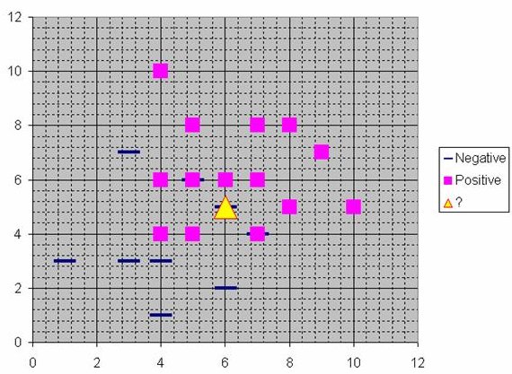
Assume that each case in the training set has two predictor variables, x and y. The cases are plotted using their x,y coordinates as shown in the figure. Also assume that the target variable has two categories, positive which is denoted by a square and negative which is denoted by a dash. Now, suppose we are trying to predict the value of a new case represented by the triangle with predictor values x=6, y=5.1. Should we predict the target as positive or negative?
Notice that the triangle is position almost exactly on top of a dash representing a negative value. But that dash is in a fairly unusual position compared to the other dashes which are clustered below the squares and left of center. So it could be that the underlying negative value is an odd case.
The nearest neighbor classification performed for this example depends on how many neighboring points are considered. If 1-NN is used and only the closest point is considered, then clearly the new point should be classified as negative since it is on top of a known negative point. On the other hand, if 9-NN classification is used and the closest 9 points are considered, then the effect of the surrounding 8 positive points may overbalance the close negative point.
A probabilistic neural network builds on this foundation and generalizes it to consider all of the other points. The distance is computed from the point being evaluated to each of the other points, and a radial basis function (RBF) (also called a kernel function) is applied to the distance to compute the weight (influence) for each point. The radial basis function is so named because the radius distance is the argument to the function.
Weight = RBF(distance)
The further some other point is from the new point, the less influence it has.
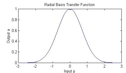
Radial Basis Function
Different types of radial basis functions could be used, but the most common is the Gaussian function:
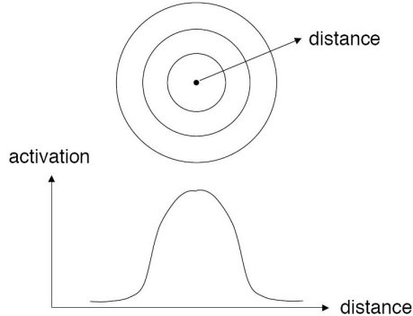
If there is more than one predictor variable, then the RBF function has as many dimensions as there are variables. Here is a RBF function for two variables:
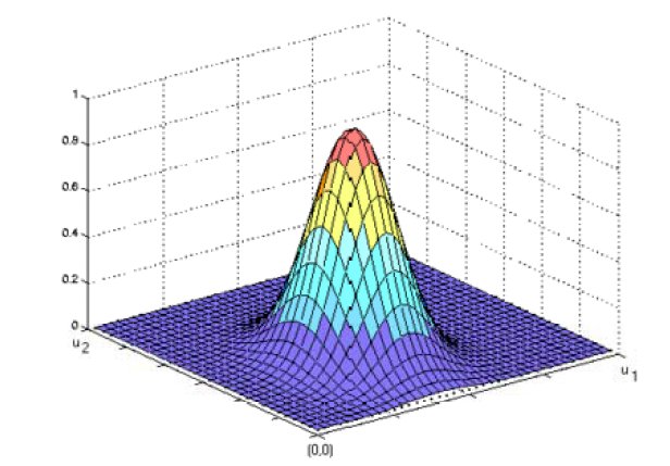
The best predicted value for the new point is found by summing the values of the other points weighted by the RBF function.
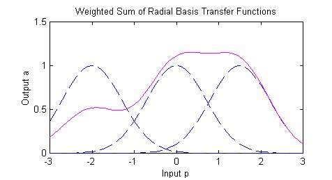
The peak of the radial basis function is always centered on the point it is weighting. The sigma value (σ) of the function determines the spread of the RBF function; that is, how quickly the function declines as the distance increased from the point.
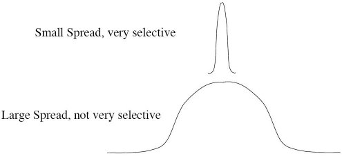
With larger sigma values and more spread, distant points have a greater influence.
The primary work of training a PNN or GRNN network is selecting the optimal sigma values to control the spread of the RBF functions. DTREG uses the conjugate gradient algorithm to compute the optimal sigma values.
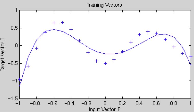
Suppose our goal is to fit the following function:
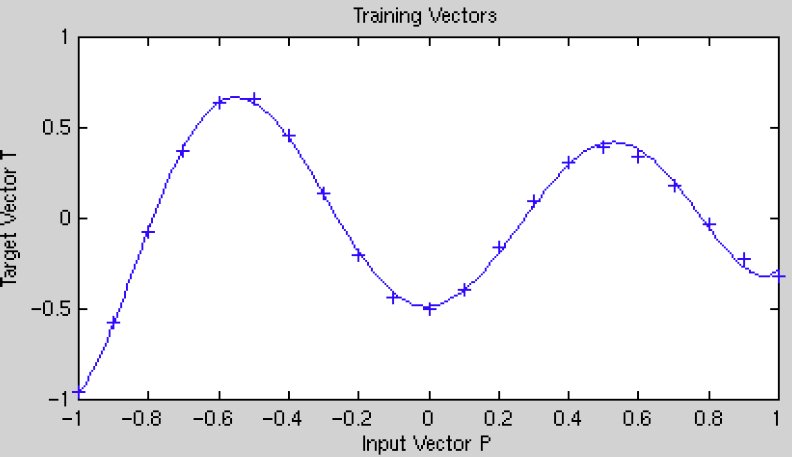
If the sigma values are too large, then the model will not be able to closely fit the function, and you will end up with a fit like this:
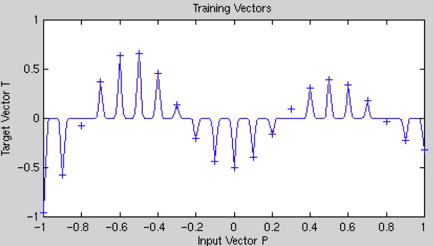
If the sigma values are too small, the model will overfit the data because each training point will have too much influence:
DTREG allows you to select whether a single sigma value should be used for the entire model, or a separate sigma for each predictor variable, or a separate sigma for each predictor variable and target category. DTREG uses the jackknife method of evaluating sigma values during the optimization process. This measures the error by building the model with all training rows except for one and then evaluating the error with the excluded row. This is repeated for all rows, and the error is averaged.
Architecture of a PNN/GRNN Network
In 1990, Donald F. Specht proposed a method to formulate the weighted-neighbor method described above in the form of a neural network. He called this a “Probabilistic Neural Network”. Here is a diagram of a PNN/GRNN network:
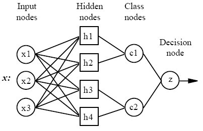
All PNN/GRNN networks have four layers:
- Input layer — There is one neuron in the input layer for each predictor variable. In the case of categorical variables, N-1 neurons are used where Nis the number of categories. The input neurons (or processing before the input layer) standardizes the range of the values by subtracting the median and dividing by the interquartile range. The input neurons then feed the values to each of the neurons in the hidden layer.
- Hidden layer — This layer has one neuron for each case in the training data set. The neuron stores the values of the predictor variables for the case along with the target value. When presented with the xvector of input values from the input layer, a hidden neuron computes the Euclidean distance of the test case from the neuron’s center point and then applies the RBF kernel function using the sigma value(s). The resulting value is passed to the neurons in the pattern layer.
- Pattern layer / Summation layer— The next layer in the network is different for PNN networks and for GRNN networks. For PNN networks there is one pattern neuron for each category of the target variable. The actual target category of each training case is stored with each hidden neuron; the weighted value coming out of a hidden neuron is fed only to the pattern neuron that corresponds to the hidden neuron’s category. The pattern neurons add the values for the class they represent (hence, it is a weighted vote for that category).
For GRNN networks, there are only two neurons in the pattern layer. One neuron is the denominator summation unit the other is the numerator summation unit. The denominator summation unit adds up the weight values coming from each of the hidden neurons. The numerator summation unit adds up the weight values multiplied by the actual target value for each hidden neuron.
- Decision layer— The decision layer is different for PNN and GRNN networks. For PNN networks, the decision layer compares the weighted votes for each target category accumulated in the pattern layer and uses the largest vote to predict the target category.
For GRNN networks, the decision layer divides the value accumulated in the numerator summation unit by the value in the denominator summation unit and uses the result as the predicted target value.
Removing unnecessary neurons
One of the disadvantages of PNN/GRNN models compared to multilayer perceptron networks is that PNN/GRNN models are large due to the fact that there is one neuron for each training row. This causes the model to run slower than multilayer perceptron networks when using scoring to predict values for new rows.
DTREG provides an option to cause it remove unnecessary neurons from the model after the model has been constructed.
Removing unnecessary neurons has three benefits:
- The size of the stored model is reduced.
- The time required to apply the model during scoring is reduced.
- Removing neurons often improves the accuracy of the model.
The process of removing unnecessary neurons is an iterative process. Leave-one-out validation is used to measure the error of the model with each neuron removed. The neuron that causes the least increase in error (or possibly the largest reduction in error) is then removed from the model. The process is repeated with the remaining neurons until the stopping criterion is reached.
When unnecessary neurons are removed, the “Model Size” section of the analysis report shows how the error changes with different numbers of neurons. You can see a graphical chart of this by clicking Chart/Model size.
There are three criteria that can be selected to guide the removal of neurons:
- Minimize error – If this option is selected, then DTREG removes neurons as long as the leave-one-out error remains constant or decreases. It stops when it finds a neuron whose removal would cause the error to increase above the minimum found.
- Minimize neurons – If this option is selected, DTREG removes neurons until the leave-one-out error would exceed the error for the model with all neurons.
- # of neurons – If this option is selected, DTREG reduces the least significant neurons until only the specified number of neurons remain.
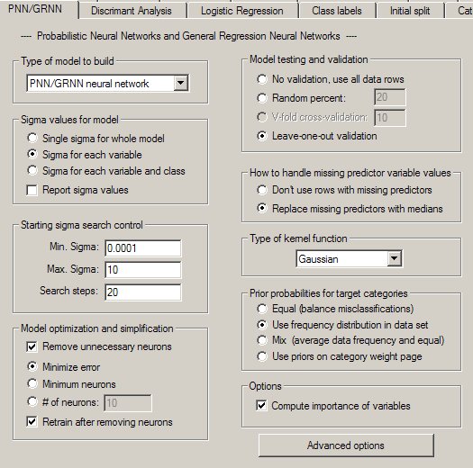
The PNN/GRNN Property Page
Controls for PNN and GRNN analyses are provided on a screen in DTREG that has the following image: