Cascade Correlation Neural Networks
Cascade correlation neural networks (Fahlman and Libiere, 1990) are “self organizing” networks. The network begins with only input and output neurons. During the training process, neurons are selected from a pool of candidates and added to the hidden layer. Cascade correlation networks have several advantages over multilayer perceptron networks:
- Because they are self organizing and grow the hidden layer during training, you do not have to be concerned with the issue of deciding how many layers and neurons to use in the network.
- Training time is very fast – often 100 times as fast as a perceptron network. This makes cascade correlation networks suitable for large training sets.
- Typically, cascade correlation networks are fairly small, often having fewer than a dozen neurons in the hidden layer. Contrast this to probabilistic neural networks which require a hidden-layer neuron for each training case.
- Cascade correlation network training is quite robust, and good results usually can be obtained with little or no adjustment of parameters.
- Cascade correlation is less likely to get trapped in local minima than multilayer perceptron networks.
As with all types of models, there are some disadvantages to cascade correlation networks:
- They have an extreme potential for overfitting the training data; this results in excellent accuracy on the training data but poor accuracy on new, unseen data. DTREG includes an overfitting control facility to prevent this.
- Cascade correlation networks usually are less accurate than probabilistic and general regression neural networks on small to medium size problems (i.e., fewer than a couple of thousand training rows). But cascade correlation scales up to handle large problems far better than probabilistic or general regression networks.
Cascade Correlation Network Architecture
A cascade correlation network consists of a cascade architecture, in which hidden neurons are added to the network one at a time and do not change after they have been added. It is called a cascade because the output from all neurons already in the network feed into new neurons. As new neurons are added to the hidden layer, the learning algorithm attempts to maximize the magnitude of the correlation between the new neuron’s output and the residual error of the network which we are trying to minimize.
A cascade correlation neural network has three layers: input, hidden and output.
Input Layer: A vector of predictor variable values (x1…xp) is presented to the input layer. The input neurons perform no action on the values other than distributing them to the neurons in the hidden and output layers. In addition to the predictor variables, there is a constant input of 1.0, called the bias that is fed to each of the hidden and output neurons; the bias is multiplied by a weight and added to the sum going into the neuron.
Hidden Layer: Arriving at a neuron in the hidden layer, the value from each input neuron is multiplied by a weight, and the resulting weighted values are added together producing a combined value. The weighted sum is fed into a transfer function, which outputs a value. The outputs from the hidden layer are distributed to the output layer.
Output Layer: For regression problems, there is only a single neuron in the output layer. For classification problems, there is a neuron for each category of the target variable. Each output neuron receives values from all of the input neurons (including the bias) and all of the hidden layer neurons. Each value presented to an output neuron is multiplied by a weight, and the resulting weighted values are added together producing a combined value. The weighted sum is fed into a transfer function, which outputs a value. The y values are the outputs of the network. For regression problems, a linear transfer function is used in the output neurons. For classification problems, a sigmoid transfer function is used.
Training Algorithm for Cascade Correlation Networks
Initially, a cascade correlation neural network consists of only the input and output layer neurons with no hidden layer neurons. Every input is connected to every output neuron by a connection with an adjustable weight, as shown below:
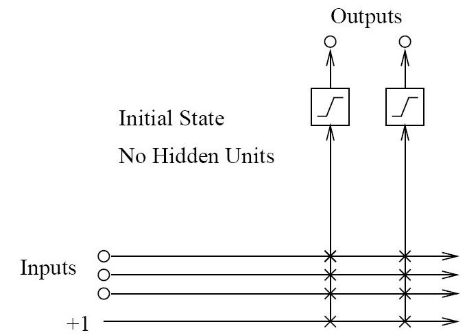
Each ‘x’ represents a weight value between the input and the output neuron. Values on a vertical line are added together after being multiplied by their weights. So each output neuron receives a weighted sum from all of the input neurons including the bias. The output neuron sends this weighted input sum through its transfer function to produce the final output.
Even a simple cascade correlation network with no hidden neurons has considerable predictive power. For a fair number of problems, a cascade correlation network with just input and output layers provides excellent predictions.
After the addition of the first hidden neuron, the network would have this structure:
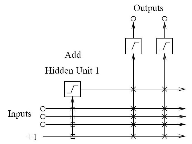
The input weights for the hidden neuron are shown as square boxes to indicate that they are fixed once the neuron has been added. Weights for the output neurons shown as ‘x’ continue to be adjustable.
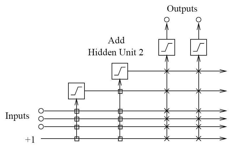
Here is a schematic of a network with two hidden neurons. Note how the second neuron receives inputs from the external inputs and pre-existing hidden neurons.
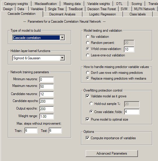
The Cascade Correlation Network Property Page
Controls for cascade correlation analyses are provided on a screen in DTREG that has the following image: