Logistic Regression

Introduction to Logistic Regression

Logistic Regression is a type of predictive model that can be used when the target variable is a categorical variable with two categories – for example live/die, has disease/doesn’t have disease, purchases product/doesn’t purchase, wins race/doesn’t win, etc. A logistic regression model does not involve decision trees and is more akin to nonlinear regression such as fitting a polynomial to a set of data values. Logistic regression can be used only with two types of target variables:

• A categorical target variable that has exactly two categories (i.e., a binary or dichotomous variable).
• A continuous target variable that has values in the range 0.0 to 1.0 representing probability values or proportions.

As an example of logistic regression, consider a study whose goal is to model the response to a drug as a function of the dose of the drug administered. The target (dependent) variable, Response, has a value 1 if the patient is successfully treated by the drug and 0 if the treatment is not successful. Thus, the general form of the model is:

Response = f(dose) The input data for Response will have the value 1 if the drug is effective and 0 if the drug is not effective. The value of Response predicted by the model represents the probability of achieving an effective outcome: P(Response=1|Dose). As with all probability values, it is in the range 0.0 to 1.0. One common question is “Why not simply use linear regression?” In fact, many studies have done just that, but there are two significant problems:

• There are no limits on the values predicted by a linear regression, so the predicted response might be less than 0 or greater than 1; clearly this is nonsensical as a response probability.
• The response usually is not a linear function of the dosage. If a minute amount of the drug is administered, no patients will respond. Doubling the dose to a larger but still minute amount will not yield any positive response. But as the dosage is increases a threshold will be reached where the drug begins to become effective. Incremental increases in the dosage above the threshold usually will elicit an increasingly positive effect. However, eventually a saturation level is reached, and beyond that point increasing the dosage does not increase the response.

The Dose-Response Curve

The logistic regression dose-response curve has an 'S' (sigmoidal) shape such as shown here:

Notice that all of the Response values are 0 or 1. The Dose varies from 0 to 25. Below a dose of 9 all of the Response values are 0. Above a dose of 10 all of the response values are 1.

The Logistic Model Formula

The logistic model formula computes the probability of the selected response as a function of the values of the predictor variables.

If a predictor variable is categorical variable with two values, then one of the values is assigned the value 1 and the other is assigned the value 0. Note that DTREG allows you to use any value for categorical variables such as “Male” and “Female”, and it converts these symbolic names into 0/1 values. So you don’t have to be concerned with recoding categorical values.

If a predictor variable is a categorical variable with more than two categories, then a separate dummy variable is generated to represent each of the categories except for one which is excluded. The value of the dummy variable is 1 if the variable has that category, and the value is 0 if the variable has any other category; hence, no more than one dummy variable will be 1. If the variable has the value of the excluded category, then all of the dummy variables generated for the variable are 0. DTREG automatically generates the dummy variables for categorical predictor variables; all you have to do is designate variables as being categorical.

In summary, the logistic formula has each continuous predictor variable, each dichotomous predictor variable with a value of 0 or 1, and a dummy variable for every category of predictor variables with more than two categories less one category. The form of the logistic model formula is:

P = 1/(1+exp(-(B0 + B1*X1 + B2*X2 + ... + Bk*Xk)))

Where B0 is a constant and Bi are coefficients of the predictor variables (or dummy variables in the case of multi-category predictor variables). The computed value, P, is a probability in the range 0 to 1. The "exp" function is e raised to a power. You can exclude the B0 constant by turning off the option “Include constant (intercept) term” on the logistic regression model property page.

Output Generated for a Logistic Regression Analysis

Summary statistics for the model

Logistic Regression Parameters

---

Predict: DeathPenalty = 1  (Yes)

Number of parameters calculated = 4

Number of data rows used = 147

Wald confidence intervals are computed for 95% probability.

Log likelihood of model = -88.142490

Deviance (-2 * Log likelihood) = 176.284981

Akaike's Information Criterion (AIC) = 184.284981

Bayesian Information Criterion (BIC) = 196.246711

The summary statistics begin by showing the name of the target variable and the category of the target whose probability is being predicted by the model.  You can select the category on the logistic regression property page for the analysis.

The log likelihood of the model is the value that is maximized by the process that computes the maximum likelihood value for the Bi parameters. 

The Deviance is equal to -2*log-likelihood.

Akaike’s Information Criterion (AIC) is -2*log-likelihood+2*k where k is the number of estimated parameters.

The Bayesian Information Criterion (BIC) is -2*log-likelihood + k*log(n) where k is the number of estimated parameters and n is the sample size.  The Bayesian Information Criterion is also known as the Schwartz criterion.

Computed Beta Parameters

  ------------------  Computed Parameter (Beta) Values  ------------------

 

   Variable      Parameter  Std. Error  Pr. Chi Sq.  Lower C.I.  Upper C.I.

--------------  ----------  ----------  -----------  ----------  ----------

BlackDefendant     0.5952      0.3939       0.1308     -0.1769      1.3673

WhiteVictim        0.2565      0.4002       0.5216     -0.5279      1.0408

Serious            0.1871      0.0612       0.0022      0.0671      0.3070

Constant          -2.6516      0.6748     < 0.0001     -3.9742     -1.3291

The computed beta parameters are the maximum likelihood values of the Bi parameters in the logistic regression model formula (see above).  By using them in an equation with the corresponding values of the predictor (X) variables, you can compute the expected probability, P, for an observation.

In addition to the maximum likelihood value, the standard error for the estimate is displayed and the Chi squared probability that the true value of the parameter is not zero.  The last two columns display the Wald upper and lower confidence intervals.  You can select the confidence interval percentage range on the Logistic Regression property page.

If a predictor variable is categorical, then a dummy variable is generated for each category except for one.  In this case, there is a Bi parameter for each dummy variable, and the categories are shown indented under the names of the variables like this:

  ---------------  Computed Parameter (Beta) Values  ---------------

Variable    Parameter  Std. Error  Pr. Chi Sq.  Lower C.I.  Upper C.I.

---------  ----------  ----------  -----------  ----------  ----------

Class

     Crew     0.8845      0.1643     < 0.0001      0.5624      1.2065

    First     1.7733      0.1896     < 0.0001      1.4016      2.1450

   Second     0.7742      0.1921     < 0.0001      0.3977      1.1507

Age

    Adult    -1.0225      0.2726       0.0002     -1.5568     -0.4881

Sex

     Male    -2.2831      0.1534     < 0.0001     -2.5838     -1.9825

Constant      1.1915      0.2765     < 0.0001      0.6495      1.7334

Likelihood Ratio Statistics

  ------  Likelihood Ratio Statistics  ------

 

   Variable      L. Ratio    DF   Pr. Chi Sq.

--------------  ----------  ----  -----------

BlackDefendant       2.321    1       0.12763

WhiteVictim          0.413    1       0.52020

Serious             10.234    1       0.00138

Constant            18.609    1       0.00002

 

If you enable the option “Compute likelihood ratio significance tests” on the logistic regression property page, then a table similar to the one shown above will be printed.  The likelihood ratio significance tests are computed by performing a logistic regression with each parameter omitted from the model and comparing the log likelihood ratio for the model with and without the parameter.  These significance tests are considered to be more reliable than the Wald significance test.  However, since the logistic regression must be recomputed with each predictor omitted, the computation time increases in proportion to the number of predictor variables.  If a predictor variable is a categorical variable with multiple categories, the significance test is performed with all of the categories included and all of them excluded.

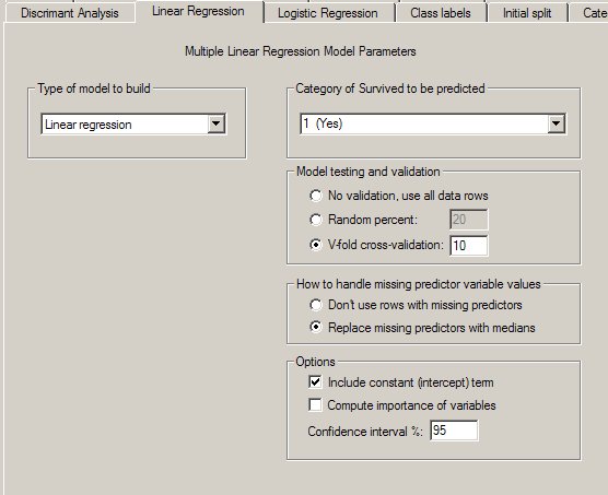
DTREG Linear Regression Control Screen

---