
GMDH Polynomial Neural Networks
Group Method of Data Handling (GMDH) polynomial neural networks are “self organizing” networks. The network begins with only input neurons. During the training process, neurons are selected from a pool of candidates and added to the hidden layers.
GMDH networks were originated in 1968 by Prof Alexey G. Ivakhnenko at the Institute of Cybernetics in Kyiv (Ukraine).
Structure of a GMDH network
GMDH networks are self organizing. This means that the connections between neurons in the network are not fixed but rather are selected during training to optimize the network. The number of layers in the network also is selected automatically to produce maximum accuracy without overfitting. The following figure from Kordik, Naplava, Snorek illustrates the structure of a basic GMDH network using polynomial functions of two variables:
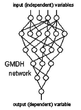
The first layer (at the top) presents one input for each predictor variable. Each neuron in the second layer draws its inputs from two of the input variables. The neurons in the third layer draw their inputs from two of the neurons in the previous layer; this progresses through each layer. The final layer (at the bottom) draws its two inputs from the previous layer and produces a single value which is the output of the network.
Inputs to neurons in GMDH networks can skip layers and come from the original variables or layers several layers earlier as illustrated by this figure:
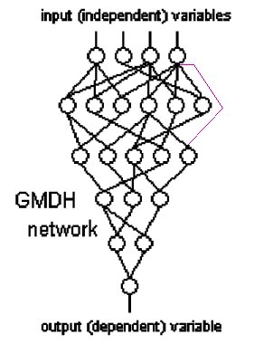
In this network, the neuron at the right end of the third layer is connected to an input variable rather than the output of a neuron on the previous layer.
Traditional GMDH neural networks use complete quadratic polynomials of two variables as transfer functions in the neurons. These polynomials have the form:
y = p0 + p1*x1 + p2*x2 + p3*x1^2 + p4*x2^2 + p5*x1*x2
DTREG extends GMDH networks by allowing you to select which functions may be used in the network.
GMDH Training Algorithm
Two sets of input data are used during the training process: (1) the primary training data, and (2) the control datawhich is used to stop the building process when overfitting occurs. The control data typically has about 20% as many rows as the training data. The percentage is specified as a training
The GMDH network training algorithm proceeds as follows:
- Construct the first layer which simply presents each of the input predictor variable values.
- Using the allowed set of functions, construct all possible functions using combinations of inputs from the previous layer. If only two-variable polynomials are enabled, there will be n*(n-1)/2 candidate neurons constructed where n is the number of neurons in the previous layer. If the option is selected to allow inputs from the previous layer and the input layer, then n will the sum of the number of neurons in the previous layer and the input layer. If the option is selected to allow inputs from any layer, then n will the sum of the number of input variables plus the number of neurons in all previous layers.
- Use least squares regression to compute the optimal parameters for the function in each candidate neuron to make it best fit the training data. Singular value decomposition (SVD) is used to avoid problems with singular matrices. If nonlinear functions are selected such as logistic or asymptotic, a nonlinear fitting routine based on Levenberg-Marquardt method is used.
- Compute the mean squared error for each neuron by applying it to the control data.
- Sort the candidate neurons in order of increasing error.
- Select the best (smallest error) neurons from the candidate set for the next layer. A model-building parameter specifies how many neurons are used in each layer.
- If the error for the best neuron in the layer as measured with the control data is better than the error from the best neuron in the previous layer, and the maximum number of layers has not been reached, then jump back to step 2 to construct the next layer. Otherwise, stop the training. Note, when overfitting begins, the error as measured with the control data will being to increase, thus stopping the training.
If you are running on a multi-core CPU system, DTREG will perform GMDH training in parallel using multiple CPU’s.
Output Generated for GMDH Networks
In addition to the usual information reported for a model, DTREG displays the actual GMDH polynomial network generated. Here is an example:
  ============  GMDH Model  ============

N(3) = 0.650821+5.931812e+012*Age{Adult}-5.931812e+012*Age{Adult}^2+4.685991e+015*Class{Second}-4.685991e+015*Class{Second}^2+0.048843*Age{Adult}*Class{Second}

N(1) = 13.82502-2.390281e+012*Class{Crew}+4.78725e+011*Class{Crew}^2-28.1043*N(3)+11.9577*N(3)^2+2.959348e+012*Class{Crew}*N(3)

N(7) = 0.325439+9.737558e+013*Sex{Male}-9.737558e+013*Sex{Male}^2+9.00077e+015*Class{Second}-9.00077e+015*Class{Second}^2+1.081648*Sex{Male}*Class{Second}

N(9) = 0.372317+2.225363e+013*Sex{Male}-2.225363e+013*Sex{Male}^2-3.960104e+015*Class{First}+3.960104e+015*Class{First}^2-0.244027*Sex{Male}*Class{First}

N(6) = -0.263746+1.221826*N(7)+0.268249*N(7)^2+1.636075*N(9)-0.172757*N(9)^2-2.019208*N(7)*N(9)

Survived{Yes} = -0.008121+1.631212*N(1)-2.485552*N(1)^2-0.186281*N(6)+0.126492*N(6)^2+1.720465*N(1)*N(6)
Output from neuron i is shown as N(i). Categorical predictor variables such as Sex are shown with the activation category in braces. For example, “Sex{Male}” has the value 1 if the value of Sex is “Male”, and it has the value 0 if Sex is any other category. The final line shows the output of the network. In this case, the probability of Survived being Yes is predicted. Note how the inputs to each neuron are drawn from the outputs of neurons in lower levels of the network. This example uses only two-variable quadratic functions.