SVM - Support Vector Machines
Introduction to Support Vector Machine (SVM) Models
A Support Vector Machine (SVM) performs classification by constructing an N-dimensional hyperplane that optimally separates the data into two categories. SVM models are closely related to neural networks. In fact, a SVM model using a sigmoid kernel function is equivalent to a two-layer, perceptron neural network.
Support Vector Machine (SVM) models are a close cousin to classical multilayer perceptron neural networks. Using a kernel function, SVM’s are an alternative training method for polynomial, radial basis function and multi-layer perceptron classifiers in which the weights of the network are found by solving a quadratic programming problem with linear constraints, rather than by solving a non-convex, unconstrained minimization problem as in standard neural network training.
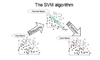
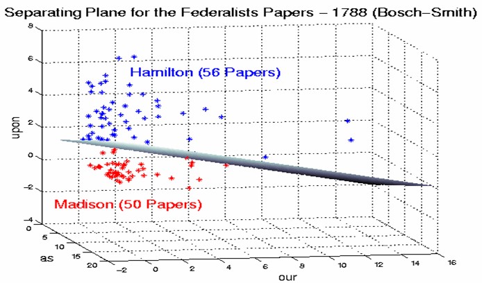
In the parlance of SVM literature, a predictor variable is called an attribute, and a transformed attribute that is used to define the hyperplane is called a feature. The task of choosing the most suitable representation is known as feature selection. A set of features that describes one case (i.e., a row of predictor values) is called a vector. So the goal of SVM modeling is to find the optimal hyperplane that separates clusters of vector in such a way that cases with one category of the target variable are on one side of the plane and cases with the other category are on the other size of the plane. The vectors near the hyperplane are the support vectors. The figure below presents an overview of the SVM process.
A Two-Dimensional Example
Before considering N-dimensional hyperplanes, let’s look at a simple 2-dimensional example. Assume we wish to perform a classification, and our data has a categorical target variable with two categories. Also assume that there are two predictor variables with continuous values. If we plot the data points using the value of one predictor on the X axis and the other on the Y axis we might end up with an image such as shown below. One category of the target variable is represented by rectangles while the other category is represented by ovals.
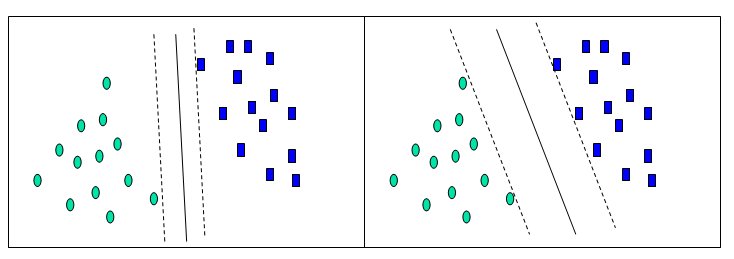
In this idealized example, the cases with one category are in the lower left corner and the cases with the other category are in the upper right corner; the cases are completely separated. The SVM analysis attempts to find a 1-dimensional hyperplane (i.e. a line) that separates the cases based on their target categories. There are an infinite number of possible lines; two candidate lines are shown above. The question is which line is better, and how do we define the optimal line.
The dashed lines drawn parallel to the separating line mark the distance between the dividing line and the closest vectors to the line. The distance between the dashed lines is called the margin. The vectors (points) that constrain the width of the margin are the support vectors. The following figure illustrates this.
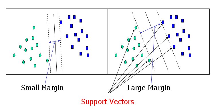
An SVM analysis finds the line (or, in general, hyperplane) that is oriented so that the margin between the support vectors is maximized. In the figure above, the line in the right panel is superior to the line in the left panel.
If all analyses consisted of two-category target variables with two predictor variables, and the cluster of points could be divided by a straight line, life would be easy. Unfortunately, this is not generally the case, so SVM must deal with (a) more than two predictor variables, (b) separating the points with non-linear curves, (c) handling the cases where clusters cannot be completely separated, and (d) handling classifications with more than two categories.
Flying High on Hyperplanes
In the previous example, we had only two predictor variables, and we were able to plot the points on a 2-dimensional plane. If we add a third predictor variable, then we can use its value for a third dimension and plot the points in a 3-dimensional cube. Points on a 2-dimensional plane can be separated by a 1-dimensional line. Similarly, points in a 3-dimensional cube can be separated by a 2-dimensional plane.
As we add additional predictor variables (attributes), the data points can be represented in N-dimensional space, and a (N-1)-dimensional hyperplane can separate them.
When Straight Lines Go Crooked
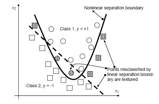
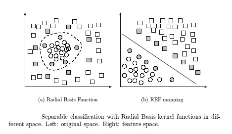
The simplest way to divide two groups is with a straight line, flat plane or an N-dimensional hyperplane. But what if the points are separated by a nonlinear region such as shown below?
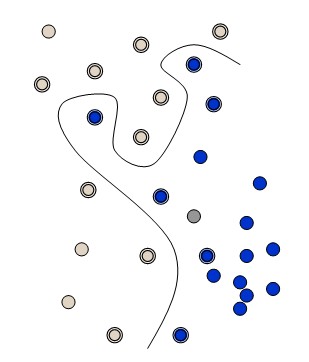
In this case we need a nonlinear dividing line.
Rather than fitting nonlinear curves to the data, SVM handles this by using a kernel function to map the data into a different space where a hyperplane can be used to do the separation.
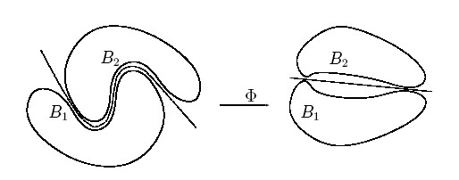
The kernel function may transform the data into a higher dimensional space to make it possible to perform the separation.
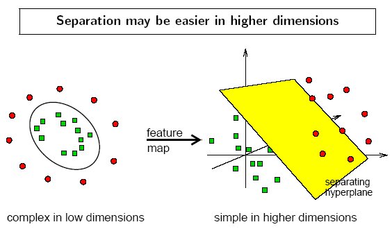
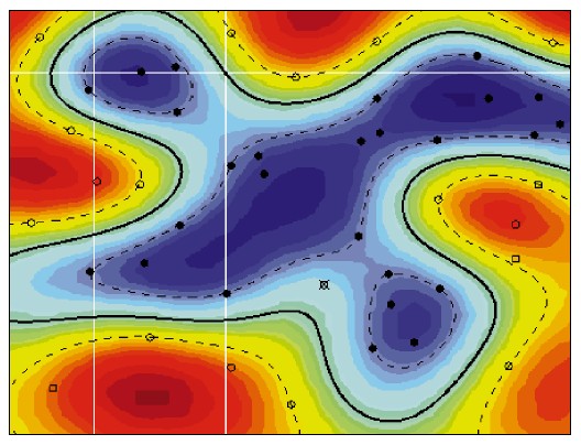
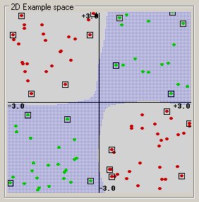
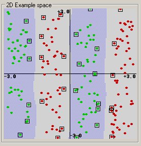
The concept of a kernel mapping function is very powerful. It allows SVM models to perform separations even with very complex boundaries such as shown below.
The Kernel Trick
Many kernel mapping functions can be used – probably an infinite number. But a few kernel functions have been found to work well in for a wide variety of applications. The default and recommended kernel function is the Radial Basis Function (RBF).
Kernel functions supported by DTREG:
Linear: u’*v
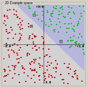
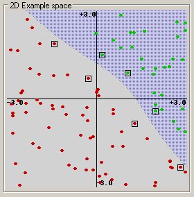
(This example was generated by pcSVMdemo.)
Polynomial: (gamma*u’*v + coef0)^degree
Radial basis function: exp(-gamma*|u-v|^2)
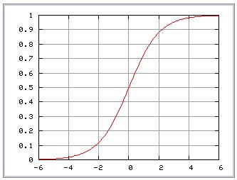
Sigmoid (feed-forward neural network): tanh(gamma*u’*v + coef0)
Parting Is Such Sweet Sorrow
Ideally an SVM analysis should produce a hyperplane that completely separates the feature vectors into two non-overlapping groups. However, perfect separation may not be possible, or it may result in a model with so many feature vector dimensions that the model does not generalize well to other data; this is known as over fitting.
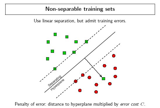
To allow some flexibility in separating the categories, SVM models have a cost parameter, C, that controls the trade off between allowing training errors and forcing rigid margins. It creates a soft margin that permits some misclassifications. Increasing the value of C increases the cost of misclassifying points and forces the creation of a more accurate model that may not generalize well. DTREG provides a grid search facility that can be used to find the optimal value of C.
Finding Optimal Parameter Values
The accuracy of an SVM model is largely dependent on the selection of the model parameters. DTREG provides two methods for finding optimal parameter values, a grid search and a pattern search. A grid search tries values of each parameter across the specified search range using geometric steps. A pattern search (also known as a “compass search” or a “line search”) starts at the center of the search range and makes trial steps in each direction for each parameter. If the fit of the model improves, the search center moves to the new point and the process is repeated. If no improvement is found, the step size is reduced and the search is tried again. The pattern search stops when the search step size is reduced to a specified tolerance.
Grid searches are computationally expensive because the model must be evaluated at many points within the grid for each parameter. For example, if a grid search is used with 10 search intervals and an RBF kernel function is used with two parameters (C and Gamma), then the model must be evaluated at 10*10 = 100 grid points. An Epsilon-SVR analysis has three parameters (C, Gamma and P) so a grid search with 10 intervals would require 10*10*10 = 1000 model evaluations. If cross-validation is used for each model evaluation, the number of actual SVM calculations would be further multiplied by the number of cross-validation folds (typically 4 to 10). For large models, this approach may be computationally infeasible.
A pattern search generally requires far fewer evaluations of the model than a grid search. Beginning at the geometric center of the search range, a pattern search makes trial steps with positive and negative step values for each parameter. If a step is found that improves the model, the center of the search is moved to that point. If no step improves the model, the step size is reduced and the process is repeated. The search terminates when the step size is reduced to a specified tolerance. The weakness of a pattern search is that it may find a local rather than global optimal point for the parameters.
DTREG allows you to use both a grid search and a pattern search. In this case the grid search is performed first. Once the grid search finishes, a pattern search is performed over a narrow search range surrounding the best point found by the grid search. Hopefully, the grid search will find a region near the global optimum point and the pattern search will then find the global optimum by starting in the right region.
Classification With More Than Two Categories
The idea of using a hyperplane to separate the feature vectors into two groups works well when there are only two target categories, but how does SVM handle the case where the target variable has more than two categories? Several approaches have been suggested, but two are the most popular: (1) “one against many” where each category is split out and all of the other categories are merged; and, (2) “one against one” where k(k-1)/2 models are constructed where k is the number of categories. DTREG uses the more accurate (but more computationally expensive) technique of “one against one”.
Optimal Fitting Without Over Fitting
The accuracy of an SVM model is largely dependent on the selection of the kernel parameters such as C, Gamma, P, etc. DTREG provides two methods for finding optimal parameter values, a grid search and a pattern search. A grid search tries values of each parameter across the specified search range using geometric steps. A pattern search (also known as a “compass search” or a “line search”) starts at the center of the search range and makes trial steps in each direction for each parameter. If the fit of the model improves, the search center moves to the new point and the process is repeated. If no improvement is found, the step size is reduced and the search is tried again. The pattern search stops when the search step size is reduced to a specified tolerance.
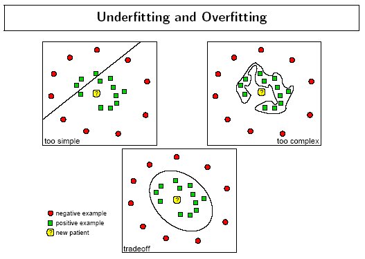
To avoid over fitting, cross-validation is used to evaluate the fitting provided by each parameter value set tried during the grid or pattern search process.
The following figure by Florian Markowetz illustrates how different parameter values may cause under or over fitting:
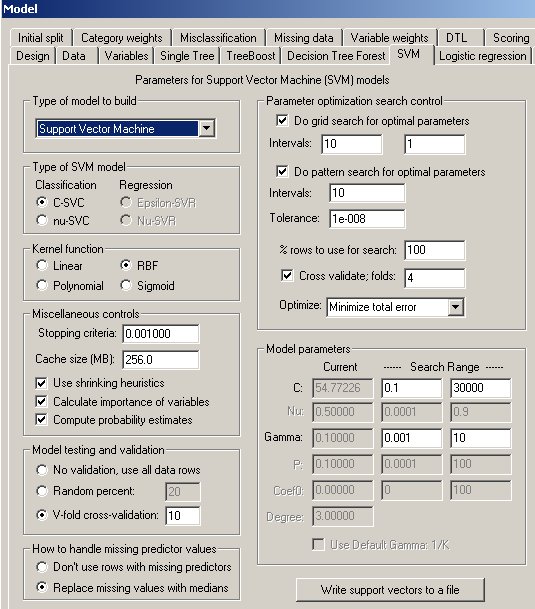
The SVM Property Page
Controls for SVM analyses are provided on a screen in DTREG that has the following image: