
Time Series Analysis
Time Series Analysis and Forecasting
"Predicting the future is hard, especially if it hasn't happened yet." -- Yogi Berra
A time series is a chronological sequence of observations on a particular variable. Usually the observations are taken at regular intervals (days, months, years), but the sampling could be irregular. Common examples of time series are the Dow Jones Industrial Average, Gross Domestic Product, unemployment rate, and airline passenger loads. A time series analysis consists of two steps: (1) building a model that represents a time series, and (2) using the model to predict (forecast) future values.
If a time series has a regular pattern, then a value of the series should be a function of previous values. If Y is the target value that we are trying to model and predict, and Yt is the value of Y at time t, then the goal is to create a model of the form:
Yt = f(Yt-1, Yt-2, Yt-3, …, Yt-n) + et
Where Yt-1 is the value of Y for the previous observation, Yt-2 is the value two observations ago, etc., and et represents noise that does not follow a predictable pattern (this is called a random shock). Values of variables occurring prior to the current observation are called lag values. If a time series follows a repeating pattern, then the value of Yt is usually highly correlated with Yt-cycle where cycle is the number of observations in the regular cycle. For example, monthly observations with an annual cycle often can be modeled by
Yt = f(Yt-12)
The goal of building a time series model is the same as the goal for other types of predictive models which is to create a model such that the error between the predicted value of the target variable and the actual value is as small as possible. The primary difference between time series models and other types of models is that lag values of the target variable are used as predictor variables, whereas traditional models use other variables as predictors, and the concept of a lag value doesn’t apply because the observations don’t represent a chronological sequence.
DTREG Time Series Analysis and Forecasting
The Enterprise Version of DTREG includes a full time series modeling and forecasting facility. Some of the features are:
- Choice of many types of base models including neural networks.
- Automatic generation of lag, moving average, slope and trend variables.
- Intervention variables
- Automatic trend removal and variance stabilization
- Autocorrelation calculation
- Validation using hold-out rows at the end of the series
- Several charts showing actual, validation, predicted, trend and residual values.
ARMA and modern types of models
Traditional time series analysis uses Box-Jenkins ARMA (Auto-Regressive Moving Average) models. An ARMA model predicts the value of the target variable as a linear function of lag values (this is the auto-regressive part) plus an effect from recent random shock values (this is the moving average part). While ARMA models are widely used, they are limited by the linear basis function.
In contrast to ARMA models, DTREG can create models for time series using neural networks, gene expression programs, support vector machines and other types of functions that can model nonlinear relationships. So, with a DTREG model, the function f(.) in
Yt = f(Yt-1, Yt-2, Yt-3, …, Yt-n) + et
can be a neural network, gene expression program or other type of general model. This makes it possible for DTREG to model time series that cannot be handled well by ARMA models.
Setting up a time series analysis
Input variables
When building a normal (not time series) model, the input must consist of values for one target variable and one or more predictor variables. When building a time series model, the input can consist of values for only a single variable – the target variable whose values are to be modeled and forecast. Here is an example of an input data set:
Passengers
112.
118.
132.
129.
121.
The time between observations must be constant (a day, month, year, etc.). If there are missing values, you must provide a row with a missing value indicator for the target variable like this:
Passengers
112.
118.
?
129.
121.
For financial data like the DJIA where there are never any values for weekend days, it is not necessary to provide missing values for weekend days. However, if there are odd missing days such as holidays, then those days must be specified as missing values. It is also desirable to put in missing values for February 29 on non-leap years so that all years have 366 observations.
Lag variables
A lag variable has the value of some other variable as it occurred some number of periods earlier. For example, here is a set of values for a variable Y, its first lag and its second lag:
Y  Y_Lag_1  Y_Lag_2
3     ?        ?
5     3        ?
8     5        3
6     8        5
Notice that lag values for observations before the beginning of the series are unknown.
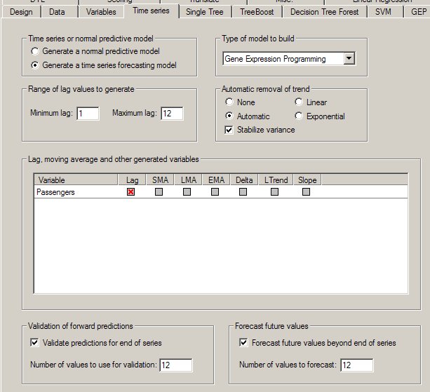
DTREG provides automatic generation of lag variables. On the Time Series Property page you can select which variables are to have lag variables generated and how far back the lag values are to run. You can also create variables for moving averages, linear trends and slopes of previous observations.
Here is an example of a Variables Property Page showing lag, moving average and other variables generated for Passengers:
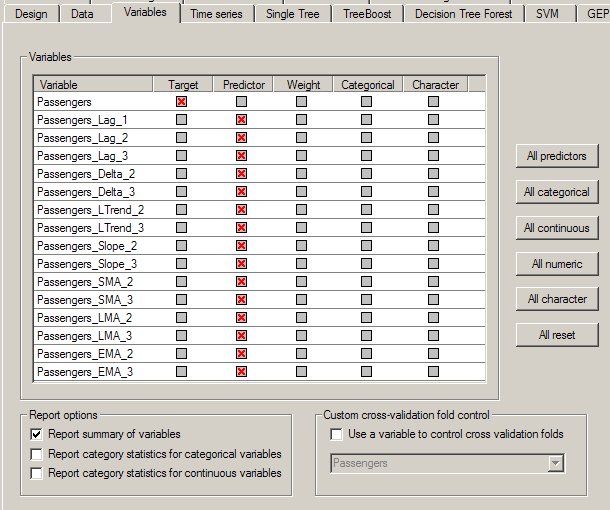
On the Variables property page, you can select which generated variables you want to use as predictors for the model. While it is tempting to generate lots of variables and use all of them in the model, sometimes better models can be generated using only lag values that are multiples of the series’ cycle period. The autocorrelation table (see below) provides information that helps to determine how many lag values are needed. Moving average, trend and slope variables may detract from the model, so you should always try building a model using only lag variables.
Intervention variables
An exceptional event occurring during a time series is known as an intervention. Examples of interventions are a change in interest rates, a terrorist act or a labor strike. Such events perturb the time series in ways that cannot be explained by previous (lag) observations.
DTREG allows you to specify additional predictor variables other than the target variable. You could have a variable for the interest rate, the gross domestic product, inflation rate, etc. You also could provide a variable with values of 0 for all rows up to the start of a labor strike, then 1 for rows during a strike, then decreasing values following the end of a strike. These variables are called intervention variables; they are specified and used as ordinary predictor variables. DTREG can generate lag values for intervention variables just as for the target variable.
Trend removal and stationary time series
A time series is said to be stationary if both its mean (the value about which it is oscillating), and its variance (amplitude) remain constant through time. Classical Box-Jenkins ARMA models only work satisfactorily with stationary time series, so for those types of models it is essential to perform transformations on the series to make it stationary. The models developed by DTREG are less sensitive to non-stationary time series than ARMA models, but they usually benefit by making the series stationary before building the model. DTREG includes facilities for removing trends from time series and adjusting the amplitude.
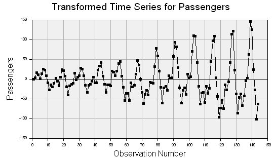
Consider this time series which has both increasing mean and variance:
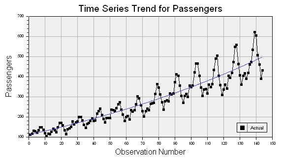
If the trend removal option is enabled on the Time Series property page (see above), then DTREG uses regression to fit either a linear or exponential function to the data. In this example, an exponential function worked best, and it is shown as the blue line running through the middle of the data points. Once the function has been fitted, DTREG subtracts it from the data values producing a new set of values that look like this:
The trend has been removed, but the variance (amplitude) is still increasing with time. If the option is enabled to stabilize variance, then the variance is adjusted to produce this series:
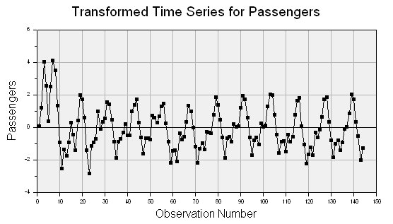
This transformed series is much closer to being stable. The transformed values are then used to build the model. A reverse transformation is applied by DTREG when making forecasts using the model.
Selecting the type of model for a time series
DTREG allows you to use the following types of models for time series:
- Decision tree
- TreeBoost (boosted series of decision trees)
- Multilayer perceptron neural network
- General regression neural network (GRNN)
- RBF neural network
- Cascade correlation network
- Support vector machine (SVM)
- Gene expression programming (GEP)
Experiments have shown that decision trees usually do not work well because they do a poor job of predicting continuous values. Gene expression programming (GEP) is an excellent method for time series because the functions generated are very general, and they can account for trends and variance changes. General regression neural networks (GRNN) also perform very well in tests. Multilayer perceptrons sometimes work very well, but they are more temperamental to train. So the best recommendation is to always try GEP and GRNN models, and then try other types of models if you have time. If you use a GEP model, it is best to enable the feature to allow it to evolve numeric constants.
Evaluating the forecasting accuracy of a model
Before you bet your life savings on the forecasts of a model, it is nice to do some tests to evaluate the predictive accuracy of the model. DTREG includes a built-in validation system that builds a model using the first observations in the series and then evaluates (validates) the model by comparing its forecast to the remaining observations at the end of the series.
Time series validation is enabled on the Time Series property page (see above).
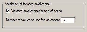
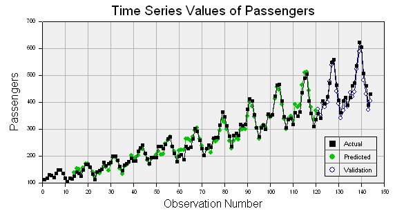
Specify the number of observations at the end of the series that you want to use for the validation. DTREG will build a model using only the observations prior to these held-out observations. It will then use that model to forecast values for the observations that were held out, and it will produce a report and chart showing the quality of the forecast. Here is an example of a chart showing the actual values with black squares and the validation forecast values with open circles:
Validation also generates a table of actual and predicted values:
 --- Validation Time Series Values ---

 Row     Actual   Predicted     Error     Error %
-----  ---------  ---------  ----------  --------
  133  417.00000  396.65452   20.345480     4.879
  134  391.00000  377.05068   13.949323     3.568
  135  419.00000  446.66871  -27.668706     6.604
  136  461.00000  435.56485   25.435146     5.517
  137  472.00000  462.14325    9.856747     2.088
  138  535.00000  517.45376   17.546240     3.280
  139  622.00000  599.82994   22.170064     3.564
  140  606.00000  611.68442   -5.684423     0.938
  141  508.00000  507.37890    0.621100     0.122
  142  461.00000  447.01704   13.982962     3.033
  143  390.00000  398.09507   -8.095074     2.076
  144  432.00000  444.67910  -12.679105     2.935
If you compare validation results from DTREG with other programs, you need to check how the other programs compute the predicted values. Some programs use actual (known) lag values when generating the predictions; this gives an unrealistically accurate prediction. DTREG uses the lag values for predicted values when forecasting: this makes validation operate like real forecasting where lag values must be based on predicted values rather than known values.
Time series model statistics report
After a model is created, DTREG produces a section in the analysis report with statistics about the model.
Autocorrelation and partial autocorrelation
The autocorrelation and partial autocorrelation tables provide important information about the significance of the lag variables.
Autocorrelation table
 -----------------------------  Autocorrelations  ------------------------------

Lag  Correlation  Std.Err.     t     -1 9 8 7 6 5 4 3 2 1 0 1 2 3 4 5 6 7 8 9 1
  1   0.70865407  0.083333    8.504  |                 .  |**************      |
  2   0.23608974  0.117980    2.001  |               .    |*****               |
  3  -0.16207088  0.121217    1.337  |               .  **|    .               |
  4  -0.41181655  0.122712    3.356  |             *******|    .               |
  5  -0.46768898  0.131961    3.544  |            ********|    .               |
  6  -0.46501203  0.143009    3.252  |            ********|     .              |
  7  -0.43595197  0.153150    2.847  |            ********|     .              |
  8  -0.36759217  0.161538    2.276  |              ******|     .              |
  9  -0.13341625  0.167246    0.798  |             .    **|      .             |
 10   0.20091610  0.167984    1.196  |             .      |****  .             |
 11   0.58898400  0.169644    3.472  |             .      |************        |
 12   0.82252315  0.183296    4.487  |             .      |****************    |
 13   0.58265202  0.207349    2.810  |            .       |************        |
 14   0.17178261  0.218423    0.786  |           .        |***     .           |
 15  -0.16852975  0.219360    0.768  |           .      **|        .           |
 16  -0.36938903  0.220257    1.677  |           .  ******|        .           |
An autocorrelation is the correlation between the target variable and lag values for the same variable. Correlation values range from -1 to +1. A value of +1 indicates that the two variables move together perfectly; a value of -1 indicates that they move in opposite directions. When building a time series model, it is important to include lag values that have large, positive autocorrelation values. Sometimes it is also useful to include those that have large negative autocorrelations. Examining the autocorrelation table shown above, we see that the highest autocorrelation is +0.82523155 which occurs with a lag of 12. Hence we want to be sure to include lag values up to 12 when building the model. It is best to experiment with including all lags from 1 to 12 and also ranges such as just 11 through 13.
DTREG computes autocorrelations for the maximum lag range specified on the Time Series property page, so you may want to set it to a large value initially to get the full autocorrelation table and then reduce it once you figure out the largest lag needed by the model.
The second column of the autocorrelation table shows the standard error of the autocorrelation, this is followed by the t-statistic in the third column.
The right side of the autocorrelation table is a bar chart with asterisks used to indicate positive or negative correlations right or left of the centerline. The dots shown in the chart mark the points two standard deviations from zero. If the autocorrelation bar is longer than the dot marker (that is, it covers it), then the autocorrelation should be considered significant. In this example, significant autocorrelations occurred for lags 1, 2, 11, 12 and 13.
Partial autocorrelation table
-------------------------  Partial Autocorrelations  --------------------------

Lag  Correlation  Std.Err.     t     -1 9 8 7 6 5 4 3 2 1 0 1 2 3 4 5 6 7 8 9 1
  1   0.70865407  0.083333    8.504  |                 .  |**************      |
  2  -0.53454362  0.083333    6.415  |          **********|  .                 |
  3  -0.11250388  0.083333    1.350  |                 . *|  .                 |
  4  -0.19447876  0.083333    2.334  |                 ***|  .                 |
  5  -0.04801434  0.083333    0.576  |                 .  |  .                 |
  6  -0.36000273  0.083333    4.320  |              ******|  .                 |
  7  -0.23338000  0.083333    2.801  |                ****|  .                 |
  8  -0.31680727  0.083333    3.802  |               *****|  .                 |
  9   0.14973536  0.083333    1.797  |                 .  |***                 |
 10  -0.03381760  0.083333    0.406  |                 .  |  .                 |
 11   0.54592233  0.083333    6.551  |                 .  |***********         |
 12   0.18345454  0.083333    2.201  |                 .  |****                |
 13  -0.45227494  0.083333    5.427  |            ********|  .                 |
 14   0.16036757  0.083333    1.924  |                 .  |***                 |
The partial autocorrelation is the autocorrelation of time series observations separated by a lag of k time units with the effects of the intervening observations eliminated.
Autocorrelation and partial autocorrelation tables are also provided for the residuals (errors) between the actual and predicted values of the time series.
Measures of fitting accuracy
DTREG generates a report with several measures of the accuracy of the predicted value. The first section compares the predicted values with the actual values for the rows use the train the model. If validation is enabled, a second table is generated showing how well the predicted validation rows match the actual rows.
============  Time Series Statistics  ============

Exponential trend: Passengers = -239.952648 + 351.737895*exp(0.005155*row)
Variance explained by trend = 86.166%
 ---  Training Data  ---

Mean target value for input data = 262.49242
Mean target value for predicted values = 261.24983

Variance in input data = 11282.932
Residual (unexplained) variance after model fit = 254.51416
Proportion of variance explained by model = 0.97744  (97.744%)

Coefficient of variation (CV) = 0.060777
Normalized mean square error (NMSE) = 0.022557
Correlation between actual and predicted = 0.988944

Maximum error = 41.131548
MSE (Mean Squared Error) = 254.51416
MAE (Mean Absolute Error) = 12.726286
MAPE (Mean Absolute Percentage Error) = 5.5055268
If DTREG removes a trend from the time series, the table shows the trend equation, and it shows how much of the total variance of the time series is explained by the trend.
There are many useful numbers in this table, but two of them are especially important for evaluating time series predictions:
Proportion of variance explained by model – this is the best single measure of how well the predicted values match the actual values. If the predicted values exactly match the actual values, then the model would explain 100% of the variance.
Correlation between actual and predicted – This is the Pearson correlation coefficient between the actual values and the predicted values; it measures whether the actual and predicted values move in the same direction. The possible range of values is -1 to +1. A positive correlation means that the actual and predicted values generally move in the same direction. A correlation of +1 means that the actual and predicted values are synchronized; this is the ideal case. A negative correlation means that the actual and predicted values move in opposite directions. A correlation near zero means that the predicted values are no better than random guesses.
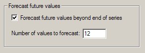
Forecasting future values
Once a model has been created for a time series, DTREG can use it to forecast future values beyond the end of the series. You enable forecasting on the Time Series property page (see above).
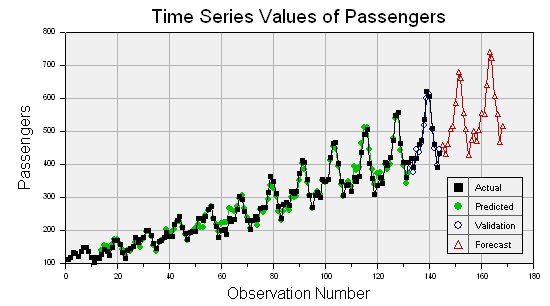
The Time Series chart displays the actual values, validation values (if validation is requested) and the forecast values.

The analysis report also displays a table of forecast values:
 --- Forecast Time Series Values ---

 Row   Predicted
-----  ---------
  145  457.63942
  146  429.32697
  147  459.64579
  148  506.19975
  149  514.89035
  150  584.91959