RBF Neural Networks
A Radial Basis Function (RBF) neural network has an input layer, a hidden layer and an output layer. The neurons in the hidden layer contain Gaussian transfer functions whose outputs are inversely proportional to the distance from the center of the neuron.
RBF networks are similar to K-Means clustering and PNN/GRNN networks. The main difference is that PNN/GRNN networks have one neuron for each point in the training file, whereas RBF networks have a variable number of neurons that is usually much less than the number of training points. For problems with small to medium size training sets, PNN/GRNN networks are usually more accurate than RBF networks, but PNN/GRNN networks are impractical for large training sets.
How RBF networks work
Although the implementation is very different, RBF neural networks are conceptually similar to K-Nearest Neighbor (k-NN) models. The basic idea is that a predicted target value of an item is likely to be about the same as other items that have close values of the predictor variables. Consider this figure:
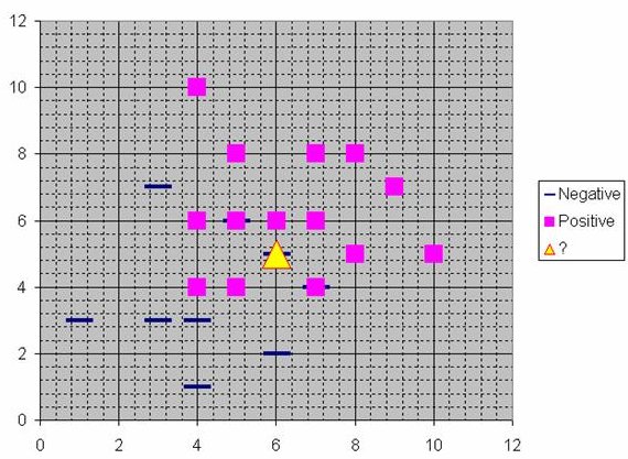
Assume that each case in the training set has two predictor variables, x and y. The cases are plotted using their x,y coordinates as shown in the figure. Also assume that the target variable has two categories, positive which is denoted by a square and negative which is denoted by a dash. Now, suppose we are trying to predict the value of a new case represented by the triangle with predictor values x=6, y=5.1. Should we predict the target as positive or negative?
Notice that the triangle is position almost exactly on top of a dash representing a negative value. But that dash is in a fairly unusual position compared to the other dashes which are clustered below the squares and left of center. So it could be that the underlying negative value is an odd case.
The nearest neighbor classification performed for this example depends on how many neighboring points are considered. If 1-NN is used and only the closest point is considered, then clearly the new point should be classified as negative since it is on top of a known negative point. On the other hand, if 9-NN classification is used and the closest 9 points are considered, then the effect of the surrounding 8 positive points may overbalance the close negative point.
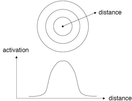
An RBF network positions one or more RBF neurons in the space described by the predictor variables (x,y in this example). This space has as many dimensions as there are predictor variables. The Euclidean distance is computed from the point being evaluated (e.g., the triangle in this figure) to the center of each neuron, and a radial basis function (RBF) (also called a kernel function) is applied to the distance to compute the weight (influence) for each neuron. The radial basis function is so named because the radius distance is the argument to the function.
Weight = RBF(distance)
The further a neuron is from the point being evaluated, the less influence it has.
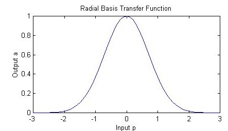
Radial Basis Function
Different types of radial basis functions could be used, but the most common is the Gaussian function:
If there is more than one predictor variable, then the RBF function has as many dimensions as there are variables. The following picture illustrates three neurons in a space with two predictor variables, X and Y. Z is the value coming out of the RBF functions:
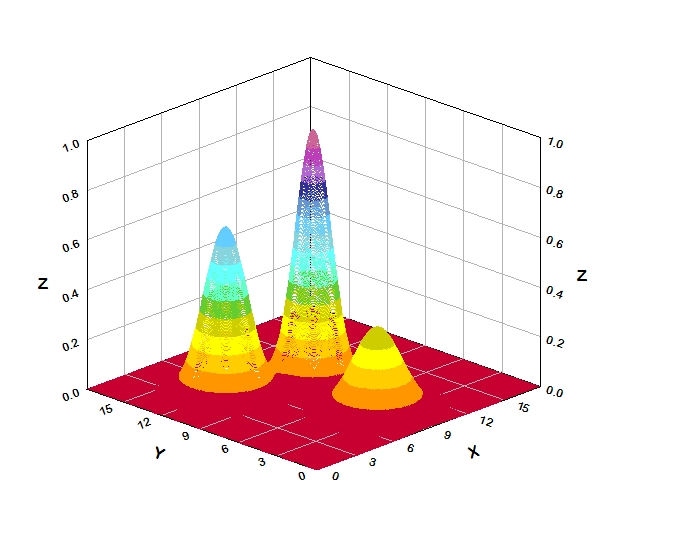
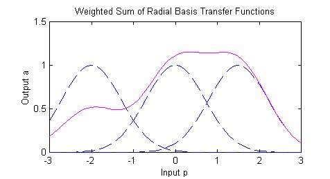
The best predicted value for the new point is found by summing the output values of the RBF functions multiplied by weights computed for each neuron.
The radial basis function for a neuron has a center and a radius (also called a spread). The radius may be different for each neuron, and, in RBF networks generated by DTREG, the radius may be different in each dimension.
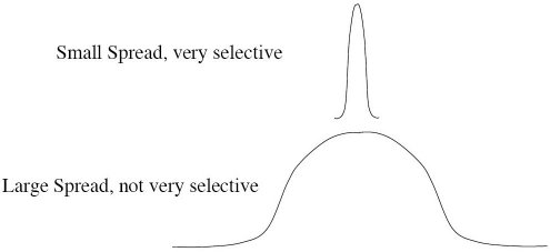
With larger spread, neurons at a distance from a point have a greater influence.
RBF Network Architecture

RBF networks have three layers:
- Input layer – There is one neuron in the input layer for each predictor variable. In the case of categorical variables, N-1 neurons are used where N is the number of categories. The input neurons (or processing before the input layer) standardizes the range of the values by subtracting the median and dividing by the interquartile range. The input neurons then feed the values to each of the neurons in the hidden layer.
- Hidden layer – This layer has a variable number of neurons (the optimal number is determined by the training process). Each neuron consists of a radial basis function centered on a point with as many dimensions as there are predictor variables. The spread (radius) of the RBF function may be different for each dimension. The centers and spreads are determined by the training process. When presented with the x vector of input values from the input layer, a hidden neuron computes the Euclidean distance of the test case from the neuron’s center point and then applies the RBF kernel function to this distance using the spread values. The resulting value is passed to the the summation layer.
- Summation layer – The value coming out of a neuron in the hidden layer is multiplied by a weight associated with the neuron (W1, W2, ...,Wn in this figure) and passed to the summation which adds up the weighted values and presents this sum as the output of the network. Not shown in this figure is a bias value of 1.0 that is multiplied by a weight W0 and fed into the summation layer. For classification problems, there is one output (and a separate set of weights and summation unit) for each target category. The value output for a category is the probability that the case being evaluated has that category.
Training RBF Networks
The following parameters are determined by the training process:
- The number of neurons in the hidden layer.
- The coordinates of the center of each hidden-layer RBF function.
- The radius (spread) of each RBF function in each dimension.
- The weights applied to the RBF function outputs as they are passed to the summation layer.
Various methods have been used to train RBF networks. One approach first uses K-means clustering to find cluster centers which are then used as the centers for the RBF functions. However, K-means clustering is a computationally intensive procedure, and it often does not generate the optimal number of centers. Another approach is to use a random subset of the training points as the centers.
DTREG uses a training algorithm developed by Sheng Chen, Xia Hong and Chris J. Harris. This algorithm uses an evolutionary approach to determine the optimal center points and spreads for each neuron. It also determines when to stop adding neurons to the network by monitoring the estimated leave-one-out (LOO) error and terminating when the LOO error beings to increase due to overfitting.
The computation of the optimal weights between the neurons in the hidden layer and the summation layer is done using ridge regression. An iterative procedure developed by Mark Orr (Orr, 1966) is used to compute the optimal regularization Lambda parameter that minimizes generalized cross-validation (GCV) error.
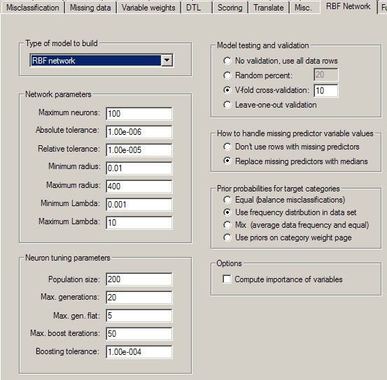
The RBF Network Property Page
Controls for RBF network analyses are provided on a screen in DTREG that has the following image: