Multilayer Perceptron Neural Networks

A Brief History of Neural Networks

Neural networks are predictive models loosely based on the action of biological neurons.

The selection of the name “neural network” was one of the great PR successes of the Twentieth Century. It certainly sounds more exciting than a technical description such as “A network of weighted, additive values with nonlinear transfer functions”. However, despite the name, neural networks are far from “thinking machines” or “artificial brains”. A typical artifical neural network might have a hundred neurons. In comparison, the human nervous system is believed to have about 3x10¹⁰ neurons. We are still light years from “Data” on Star Trek.

The original “Perceptron” model was developed by Frank Rosenblatt in 1958. Rosenblatt’s model consisted of three layers, (1) a “retina” that distributed inputs to the second layer, (2) “association units” that combine the inputs with weights and trigger a threshold step function which feeds to the output layer, (3) the output layer which combines the values. Unfortunately, the use of a step function in the neurons made the perceptions difficult or impossible to train. A critical analysis of perceptrons published in 1969 by Marvin Minsky and Seymore Papert pointed out a number of critical weaknesses of perceptrons, and, for a period of time, interest in perceptrons waned.

Interest in neural networks was revived in 1986 when David Rumelhart, Geoffrey Hinton and Ronald Williams published “Learning Internal Representations by Error Propagation”. They proposed a multilayer neural network with nonlinear but differentiable transfer functions that avoided the pitfalls of the original perceptron’s step functions. They also provided a reasonably effective training algorithm for neural networks.

Types of Neural Networks

When used without qualification, the terms “Neural Network” (NN) and “Artificial Neural Network” (ANN) usually refer to a Multilayer Perceptron Network. However, there are many other types of neural networks including Probabilistic Neural Networks, General Regression Neural Networks, Radial Basis Function Networks, Cascade Correlation, Functional Link Networks, Kohonen networks, Gram-Charlier networks, Learning Vector Quantization, Hebb networks, Adaline networks, Heteroassociative networks, Recurrent Networks and Hybrid Networks.

DTREG implements the most widely used types of neural networks: Multilayer Perceptron Networks (also known as multilayer feed-forward network), Cascade Correlation Neural Networks, Probabilistic Neural Networks (PNN) and General Regression Neural Networks (GRNN). This section describes Multilayer Perceptron Networks. Click here for information about Probabilistic and General Regression neural networks. Click here for information about Cascade Correlation neural networks.

The Multilayer Perceptron Neural Network Model

The following diagram illustrates a perceptron network with three layers:

 

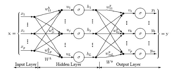
This network has an input layer (on the left) with three neurons, one hidden layer (in the middle) with three neurons and an output layer (on the right) with three neurons.

There is one neuron in the input layer for each predictor variable. In the case of categorical variables, N-1 neurons are used to represent the N categories of the variable.

Input Layer — A vector of predictor variable values (x₁...x_p) is presented to the input layer. The input layer (or processing before the input layer) standardizes these values so that the range of each variable is -1 to 1. The input layer distributes the values to each of the neurons in the hidden layer. In addition to the predictor variables, there is a constant input of 1.0, called the bias that is fed to each of the hidden layers; the bias is multiplied by a weight and added to the sum going into the neuron.

Hidden Layer — Arriving at a neuron in the hidden layer, the value from each input neuron is multiplied by a weight (w_ji), and the resulting weighted values are added together producing a combined value u_j. The weighted sum (u_j) is fed into a transfer function, σ, which outputs a value h_j. The outputs from the hidden layer are distributed to the output layer.

Output Layer — Arriving at a neuron in the output layer, the value from each hidden layer neuron is multiplied by a weight (w_kj), and the resulting weighted values are added together producing a combined value v_j. The weighted sum (v_j) is fed into a transfer function, σ, which outputs a value y_k. The y values are the outputs of the network.

If a regression analysis is being performed with a continuous target variable, then there is a single neuron in the output layer, and it generates a single y value. For classification problems with categorical target variables, there are N neurons in the output layer producing N values, one for each of the N categories of the target variable.

Multilayer Perceptron Architecture

The network diagram shown above is a full-connected, three layer, feed-forward, perceptron neural network. “Fully connected” means that the output from each input and hidden neuron is distributed to all of the neurons in the following layer. “Feed forward” means that the values only move from input to hidden to output layers; no values are fed back to earlier layers (a Recurrent Network allows values to be fed backward).

All neural networks have an input layer and an output layer, but the number of hidden layers may vary. Here is a diagram of a perceptron network with two hidden layers and four total layers:

 

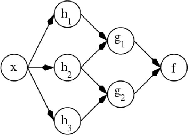
When there is more than one hidden layer, the output from one hidden layer is fed into the next hidden layer and separate weights are applied to the sum going into each layer.

Training Multilayer Perceptron Networks

The goal of the training process is to find the set of weight values that will cause the output from the neural network to match the actual target values as closely as possible. There are several issues involved in designing and training a multilayer perceptron network:

• Selecting how many hidden layers to use in the network.
• Deciding how many neurons to use in each hidden layer.
• Finding a globally optimal solution that avoids local minima.
• Converging to an optimal solution in a reasonable period of time.
• Validating the neural network to test for overfitting.

Selecting the Number of Hidden Layers

For nearly all problems, one hidden layer is sufficient. Two hidden layers are required for modeling data with discontinuities such as a saw tooth wave pattern. Using two hidden layers rarely improves the model, and it may introduce a greater risk of converging to a local minima. There is no theoretical reason for using more than two hidden layers. DTREG can build models with one or two hidden layers. Three layer models with one hidden layer are recommended.

Deciding how many neurons to use in the hidden layers

One of the most important characteristics of a perceptron network is the number of neurons in the hidden layer(s). If an inadequate number of neurons are used, the network will be unable to model complex data, and the resulting fit will be poor.

If too many neurons are used, the training time may become excessively long, and, worse, the network may over fit the data. When overfitting occurs, the network will begin to model random noise in the data. The result is that the model fits the training data extremely well, but it generalizes poorly to new, unseen data. Validation must be used to test for this.

DTREG includes an automated feature to find the optimal number of neurons in the hidden layer. You specify the minimum and maximum number of neurons you want it to test, and it will build models using varying numbers of neurons and measure the quality using either cross validation or hold-out data not used for training. This is a highly effective method for finding the optimal number of neurons, but it is computationally expensive, because many models must be built, and each model has to be validated. If you have a multiprocessor computer, you can configure DTREG to use multiple CPU’s during the process.

The automated search for the optimal number of neurons only searches the first hidden layer. If you select a model with two hidden layers, you must manually specify the number of neurons in the second hidden layer.

Finding a globally optimal solution

A typical neural network might have a couple of hundred weighs whose values must be found to produce an optimal solution. If neural networks were linear models like linear regression, it would be a breeze to find the optimal set of weights. But the output of a neural network as a function of the inputs is often highly nonlinear; this makes the optimization process complex.

If you plotted the error as a function of the weights, you would likely see a rough surface with many local minima such as this:

 

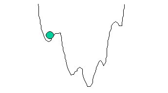
This picture is highly simplified because it represents only a single weight value (on the horizontal axis). With a typical neural network, you would have a 200-dimension, rough surface with many local valleys.

Optimization methods such as steepest descent and conjugate gradient are highly susceptible to finding local minima if they begin the search in a valley near a local minimum. They have no ability to see the big picture and find the global minimum.

Several methods have been tried to avoid local minima. The simplest is just to try a number of random starting points and use the one with the best value. A more sophisticated technique called simulated annealing improves on this by trying widely separated random values and then gradually reducing (“cooling”) the random jumps in the hope that the location is getting closer to the global minimum.

DTREG uses the Nguyen-Widrow algorithm to select the initial range of starting weight values. It then uses the conjugate gradient algorithm to optimize the weights. Conjugate gradient usually finds the optimum weights quickly, but there is no guarantee that the weight values it finds are globally optimal. So it is useful to allow DTREG to try the optimization multiple times with different sets of initial random weight values. The number of tries allowed is specified on the Multilayer Perceptron property page.

Converging to the Optimal Solution — Conjugate Gradient

Given a set of randomly-selected starting weight values, DTREG uses the conjugate gradient algorithm to optimize the weight values.

Most training algorithms follow this cycle to refine the weight values: (1) run a set of predictor variable values through the network using a tentative set of weights, (2) compute the difference between the predicted target value and the actual target value for this case, (3) average the error information over the entire set of training cases, (4) propagate the error backward through the network and compute the gradient (vector of derivatives) of the change in error with respect to changes in weight values, (5) make adjustments to the weights to reduce the error. Each cycle is called an epoch.

Because the error information is propagated backward through the network, this type of training method is called backward propagation.

The backpropagation training algorithm was first described by Rumelhart and McClelland in 1986; it was the first practical method for training neural networks. The original procedure used the gradient descent algorithm to adjust the weights toward convergence using the gradient. Because of this history, the term “backpropagation” or “backprop” often is used to denote a neural network training algorithm using gradient descent as the core algorithm. That is somewhat unfortunate since backward propagation of error information through the network is used by nearly all training algorithms, some of which are much better than gradient descent.

Backpropagation using gradient descent often converges very slowly or not at all. On large-scale problems its success depends on user-specified learning rate and momentum parameters. There is no automatic way to select these parameters, and if incorrect values are specified the convergence may be exceedingly slow, or it may not converge at all. While backpropagation with gradient descent is still used in many neural network programs, it is no longer considered to be the best or fastest algorithm.

DTREG uses the conjugate gradient algorithm to adjust weight values using the gradient during the backward propagation of errors through the network. Compared to gradient descent, the conjugate gradient algorithm takes a more direct path to the optimal set of weight values. Usually, conjugate gradient is significantly faster and more robust than gradient descent. Conjugate gradient also does not require the user to specify learning rate and momentum parameters.

The traditional conjugate gradient algorithm uses the gradient to compute a search direction. It then uses a line search algorithm such as Brent’s Method to find the optimal step size along a line in the search direction. The line search avoids the need to compute the Hessian matrix of second derivatives, but it requires computing the error at multiple points along the line. The conjugate gradient algorithm with line search (CGL) has been used successfully in many neural network programs, and is considered one of the best methods yet invented.

DTREG provides the traditional conjugate gradient algorithm with line search, but it also offers a newer algorithm, Scaled Conjugate Gradient developed in 1993 by Martin Fodslette Moller.

The scaled conjugate gradient algorithm uses a numerical approximation for the second derivatives (Hessian matrix), but it avoids instability by combining the model-trust region approach from the Levenberg-Marquardt algorithm with the conjugate gradient approach. This allows scaled conjugate gradient to compute the optimal step size in the search direction without having to perform the computationally expensive line search used by the traditional conjugate gradient algorithm. Of course, there is a cost involved in estimating the second derivatives.

Tests performed by Moller show the scaled conjugate gradient algorithm converging up to twice as fast as traditional conjugate gradient and up to 20 times as fast as backpropagation using gradient descent. Moller’s tests also showed that scaled conjugate gradient failed to converge less often than traditional conjugate gradient or backpropagation using gradient descent.

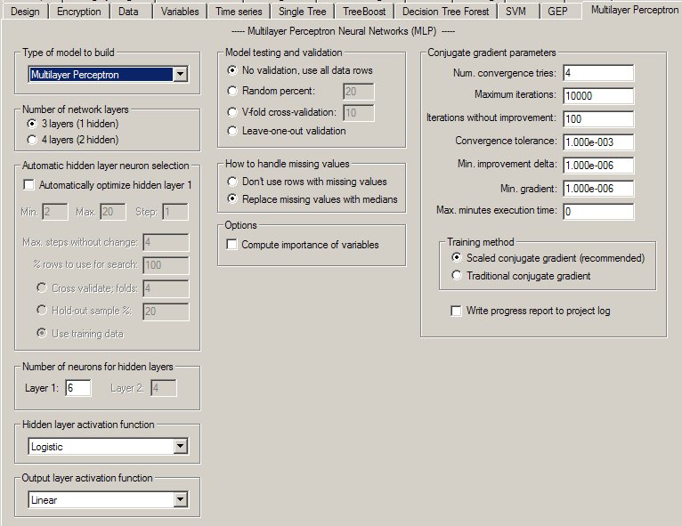
The Multilayer Perceptron Property Page

Controls for multilayer perceptron analyses are provided on a screen in DTREG that has the following image: