Gene Expression Programming

Gene Expression Programming is a procedure that mimics biological evolution to create a computer program to model some phenomenon. Gene expression programming can be used to create many different types of models including decision trees, neural networks and polynomial constructs. The type of gene expression programming implemented in DTREG is Symbolic Regression – so named because it creates a symbolic mathematical or logical function.

DTREG provides a full implementation of the Gene Expression Programming algorithm developed by Cândida Ferreira. Here are some of the features of DTREG’s implementation:

Continuous and categorical target variables
Automatic handling of categorical predictor variables
A large library of functions that you can select for inclusion in the model
Mathematical and logical (AND, OR, NOT, etc.) function generation
Choice of many fitness functions
Both static linking functions and evolving homeotic genes
Fixed and random constants
Nonlinear regression to optimize constants
Parsimony pressure to optimize the size of functions
Automatic algebraic simplification of the combined function
Several forms of validation including cross-validation and hold-out
Computation of the relative importance of predictor variables
Automatic generation of C or C++ source code for the functions
Multi-CPU execution for multiple target categories and cross-validation

Symbolic Regression

In ordinary mathematical regression, the procedure is given the form of the function to be fitted to the data. This could be a linear function for linear regression or a general mathematical function for nonlinear regression. The regression procedure computes the optimal values of parameters for the function to make the function fit a data set as well as possible, but the regression procedure does not alter the form of the function. For example, a linear regression problem with two variables has the form:

y = a+b*x

Where x is the independent variable, y is the dependent variable, and a and b are parameters whose values are to be computed by the regression algorithm. This type of procedure is classified as parametric regression, because the goal is to estimate parameters for a function whose form is known (or assumed).

With nonparametric regression the form of the function is not known in advance, and it is the goal of the procedure to find a function that will fit the data. So we are looking for f(·) that will best fit

y=f(x₁,x₂,…,x_n)

Where y is the dependent variable and there are n independent x variables.

There are many possible forms of nonparametric functions – neural networks and decision trees are types of nonparametric functions. Symbolic regression is a subset of nonparametric regression that restricts the functions to be mathematical or logical expressions.

Symbolic Regression Example – Kepler’s Third Law

Around 1605, the German mathematician and astronomer Johannes Kepler discovered three astronomical laws that describe the orbits of planets around the Sun. Kepler’s work was based on the precise astronomical observations recorded by Danish astronomer Tycho Brahe. Kepler’s third law states “The squares of the orbital periods of planets are directly proportional to the cubes of the semi-major axis of the orbits.” Mathematically, this is:

Period² = constant*Distance³

Let’s see if symbolic regression can figure this out without the help of a genius astronomer. We will use the following data as input to the procedure:

Planet	Distance	Period
Venus	0.72	0.61
Earth	1.00	1.00
Mars	1.52	1.84
Jupiter	5.20	11.90
Saturn	9.53	29.40
Uranus	19.10	83.50

Gene expression programming was used to model this data. Two genes were used per chromosome, and there were 7 symbols in the head section of each gene. After four generations, DTREG found a perfect fit to the data. The expression generated and displayed by DTREG is:

Period = sqrt(Distance)*Distance

Simplifying this we find:

Period = sqrt(Distance)*Distance
Period = Distance^(3/2)
Period² = Distance³

This is exactly Kepler’s third law.

Odd Parity Example

In this example, symbolic regression will be used to find a logical expression to compute the parity for a 3-input binary circuit. The output parity value should be 1 if there are an odd number of inputs with the value 1, and the output should be 0 if there are an even number of inputs with the value 1. Here is the data for the analysis:

In1	In2	In3	Parity
0	0	0	0
0	0	1	1
0	1	0	1
0	1	1	0
1	0	0	1
1	0	1	0
1	1	0	0
1	1	1	1

For this problem we will allow DTREG to use only three functions in the expression: AND, OR, NOT. We will use 3 genes per chromosome, and we will use the AND function to link the genes. After 418 generations to train the model and an additional 397 generations to simplify it, DTREG generated the following function which perfectly fits the data:

Parity = (In3|(!(In1&In2)))&((!(In1|In2))|(In1&In2)|!In3)&In2|(In1|In3)

Where ‘|’ is the OR operator, ‘&’ is AND, and ‘!’ is NOT.

Genetic Algorithms

Genetic algorithms (GA) have been in widespread use since the 1980’s, but the first experiments with computer simulated evolution go back to 1954.

Genetic algorithms are basically a smart search procedure. The goal is to find a solution in a multi-dimensional space where there is no known exact algorithm. Genetic algorithms are often thousands or even millions of times faster than exhaustive search procedures. Exhaustive search is impractical for high dimension problems. The use of random mutations allows genetic algorithms to avoid being trapped in locally-optimal regions which is a serious problem for hill-climbing algorithms typically used for iterative/convergence procedures. Genetic algorithms have been used to solve otherwise intractable problems such as the Traveling Salesperson Problem.

Genetic algorithms mimic biological evolution, and the terms used for genetic algorithms are based on biological features.

In biological DNA systems, the basic units are the adenine (A), thymine (T), guanine (G) and cytosine (C) nucleotides that join the helical strands. In genetic algorithms, the basic unit is called a symbol. The nature of symbols depends on the particular genetic algorithm. In gene expression programming, the symbols consist of functions, variables and constants. Symbols for variables and constants are called terminals, because they have no arguments.

An ordered set of symbols form a gene, and an ordered set of genes form a chromosome. In GEP programs, genes typically have 4 to 20 symbols, and chromosomes are typically built from 2 to 10 genes; chromosomes may consist of only a single gene. The DNA strand for a mammal typically contains about 5x10⁹ nucleotides.

Genetic Algorithms for Symbolic Regression

Many efforts have been made to use genetic algorithms to solve symbolic regression problems – that is, to generate symbolic functions to model data. One of the problems that plagues most of the efforts is finding a way to efficiently mutate and cross-breed symbolic expressions so that the resulting expressions have a valid mathematical syntax. For example, if you mutate (2*x+3) into (x 2+3*) it isn’t any good, because it isn’t syntactically correct.

One approach to this problem is to perform a mutation, check the result and then try a different random mutation until a syntactically valid expression is generated. Obviously, this can be a time consuming process for complex expressions.

A second approach is to limit what type of mutations can be performed – for example, only exchanging complete sub-expressions. The problem with this approach is that if limited mutations are used, the evolution process is hindered, and it may take a large number of generations to find a solution, or it may be completely unable to find the optimal solution.

Gene Expression Programming

An elegant and efficient solution to the expression-mutation problem was discovered in 1999 by Cândida Ferreira (Ferreira 1996). Ferreira devised a system for encoding expressions that allows fast application of a wide variety of mutation and cross-breeding techniques while guaranteeing that the resulting expression will always be syntactically valid. This approach is called Gene Expression Programming (GEP). Experiments have shown that GEP is 100 to 60,000 times faster than older genetic algorithms.

Expression Trees and Karva

The key to GEP’s ability to quickly mutate valid expressions is the way it encodes symbols in genes. This notation is called the Karva Language. Expressions encoded using Karva are called K-expressions. Consider the simple mathematical expression:

a*b+c

This can be encoded as an expression tree of the form

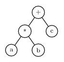
An expression tree is an excellent way to represent an expression in a computer, because the tree can be arbitrarily complex, and expression trees can be evaluated quickly.

To convert an expression tree to the Karva notation, start at the left-most symbol in the top line of the tree and scan symbols left-to-right and top-to-bottom. Each time a symbol is encountered, add it to the K-expression in left-to-right order. When there are no more symbols on a line, advance to the left end of the following line. Using this method, the tree shown above is converted to the K-expression:

+*cab

Note that + is the first symbol found on the first line, at the end of that line scanning begins on the second line and finds * followed by c. It then starts with the third line and finds a and b.

As a second example, consider the expression a*b+sqrt(c*d) The corresponding expression tree is

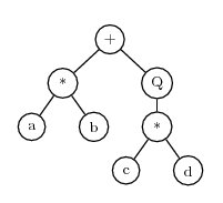
Where ‘Q’ represents square root. This can be translated to the K-expression

+*Qab*cd

The process of converting an expression tree to a K-expression can be carried out quickly by a computer. A reverse process can quickly convert a K-expression back to an expression tree.

Genes

A gene consists of a fixed number of symbols encoded in the Karva language. A gene has two sections, the head and the tail. The head is used to encode functions for the expression. The tail is a reservoir of extra terminal symbols that can be used if there aren’t enough terminals in the head to provide arguments for the functions. Thus, the head can contain functions, variables and constants, but the tail can contain only variables and constants (i.e. terminals). The number of symbols in the head of a gene is specified as a parameter for the analysis. The number of symbols in the tail is determined by the equation

t = h*(MaxArg-1)+1

Where t is the number of symbols in the tail, h is the number of symbols in the head, and MaxArg is the maximum number of arguments required by any function that is allowed to be used in the expression. For example, if the head length is 6 and the allowable set of functions consists of binary operators (+, -, *, /), then the tail length is:

t = 6*(2-1)+1 = 7

The purpose of the tail is to provide a reservoir of terminal symbols (variables and constants) that can be used as arguments for functions in the head if there aren’t enough terminals in the head.

Consider a gene with three symbols in the head and which uses binary arithmetic operators. The tail will then have 3*(2-1)+1=4 terminal symbols. Here is an example of such a gene. The head is in front of the comma, and the tail follows the comma:

+-/,abcd

Ignoring the distinction between the head and the tail, this K-expression can be converted to this expression tree:

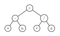
Note that the head of the gene consisted only of functions, but the tail provided enough terminals to fill in the arguments for the functions.

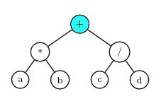
During mutation, symbols in the head can be replaced by either function or terminal symbols. Symbols in the tail can be replaced only by terminals. Using the same example K-expression shown above, assume mutation replaces the ‘/’ symbol with d. Then the K-expression is:

+-d,abcd

And the expression tree becomes

Note that this expression tree has fewer nodes than the previous one. This illustrates an important point: by allowing mutation to replace functions with terminals and terminals with functions, the size of the expression can change was well as its content. As a further example, assume the next mutation changes the first symbol in the K-expression from ‘+’ to c. The K-expression becomes:

c-d,abcd

The expression tree for this is:

The “tree” consists of a single node which is the variable c. Note that the number of symbols in the gene did not change, but some symbols are not used. The symbols that are not used are called the noncoding region of the gene. Because the functional length of a gene may be less than the number of symbols it holds, it is called an open reading frame (ORF). Biological genes also have noncoding regions.

If you experiment with K-expressions you will find that any possible mutation will result in a valid expression as long as the following rules are adhered to:

Symbols in the head can be replaced with functions, variables and constants.
Symbols in the tail can be replaced only with variables and constants (terminals).
The tail is of sufficient length to provide terminals for all possible functions that can occur in the head. (See the formula for tail length above.)

This is the key to the efficiency of gene expression programming. It is easy for a computer program to follow these three rules while performing mutations, and it never has to check whether the resulting expression has valid syntax. By allowing a broad range of mutations, the process can efficiently explore a high dimensional space, and the expressions can change in size as functions are replaced by terminals and terminals by functions.

Chromosomes and Linking Functions

A chromosome consists of one or more genes. The number of genes in a chromosome is a parameter for the analysis. If there is more than one gene in a chromosome, then a linking function is used to join the genes in the final function. The linking function can be static or evolving.

For example, consider a chromosome with two genes having the K-expressions:

Gene 1: *ab
Gene 2: /cd

If ‘+’ is used as the static linking function, then the combined expression is:

Which is equivalent to (a*b+c/d).

Homeotic Genes

In addition to specifying a static linking function, you can allow the linking functions to be selected dynamically by evolution. This is done using homeotic genes.

In biology, homeotic genes control macro organization such as determining that arms should be attached to shoulders and legs to hips. Mutations in homeotic genes produce bizarre creatures. An example is the Antennapedia mutant of the fruit fly Drosophila, where legs are found sprouting where the antennae would normally be. Often, mutations in homeotic genes produce nonviable organisms.

In gene expression programming, a homeotic gene is used to link together the regular genes in a chromosome. There is never more than one homeotic gene in a chromosome, and there is no homeotic gene if a static linking function is used.

Homeotic genes have the same structure as regular genes: They have a head section with a length specified as a parameter, a tail section, and a set of symbols. The symbols in homeotic genes consist of references to ordinary genes and linking functions.

Homeotic genes undergo mutation, inversion, transposition and crossover just as regular genes do during evolution. Separate parameters are available to set the mutation rates for homeotic genes. Symbols and functions are never exchanged between regular genes and homeotic genes.

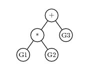
For example, if a chromosome has 3 regular genes, G1, G2 and G3, and a homeotic gene, then the homeotic gene might have a K-expression of

+*G3G1G2

And the expression tree would be

Mathematical Evolution

Evolution is the engine of gene expression programming. An initial population of candidate functions is created, then mutation, breeding and natural selection are used to evolve functions that more closely model the data.

The main steps in the training and evolution of a gene expression program are:

Create an initial population of viable individuals (chromosomes).
Use evolution to attempt to create individuals that fit the data well.
Use evolution to try to find a simpler, more parsimonious function.
Use nonlinear regression to find optimal values of constants.

Initial Population Creation

Gene expression programming and other genetic algorithms work by evolving sets of individuals (chromosomes). But before the evolution process begins, an initial, founder population of individuals must be constructed that can mutate, breed and be selected for subsequent generations. The number of individuals in the population is a parameter for the analysis.

The Karva language used to represent expressions in gene expression programming guarantees that all expressions will have valid mathematical syntax. But Karva does not guarantee that the expressions will produce meaningful values when they are evaluated. For example, the K-expression

/a0

is syntactically valid, but it generates the expression (a/0), which, of course, is infinite. There are many other cases where the results cannot be evaluated such as taking the square root of a negative number, finding the log of a negative number or overflowing the range of numbers by raising a large value to a huge power. Expressions that cannot be evaluated to generate meaning values are called unviable and receive a fitness score of zero. Expressions are also classified as unviable if they are unable to correctly classify any members of the population. Some fitness functions place additional conditions on viability: For example, the Hits with penalty fitness function only classifies an expression as viable if both the true positive (TP) and true negative (TN) hit counts are greater than zero.

The creation of the initial population is done by randomly selecting functions and terminals for the genes. Some of the resulting individuals may be viable, and some may be unviable. If the population has no viable individuals, another population is randomly created. This process is repeated up to several thousand times until an initial population is found with at least one viable individual. If it is impossible to create an initial population with a viable individual, then the analysis cannot be performed.

The Process of Evolution

Once the initial population has been created, the process of evolution can be used to find individuals that model the data well. Here is an outline of the evolution process:

Convert K-expressions in chromosomes to expression trees.
Compute the fitness score for each individual by comparing the predicted target value with the actual target value for all training cases.
If the fitness score is sufficiently good, or if the maximum number of generations has been evolved, or if the maximum execution time has been reached, stop the evolution.
Transfer the best (most fit) individual to the next generation without modification.
Use roulette-wheel sampling to select individuals for the next generation.
Perform mutations.
Perform inversions.
Perform transposition.
Perform recombination to combine genetic material from pairs of individuals.
Return to step 1 for the next evolution cycle.

Natural Selection and Fitness

The principle of natural selection is that healthy, fit individuals should breed and produce offspring at a faster rate than sick, unfit individuals. Through this selection process, each generation becomes healthier and more fit. In order for this to take place, there must be some characteristics of individuals that determine fitness for the environment, and there must be a selection mechanism that favors the breeding of individuals with greater fitness.

In gene expression programming, fitness is based on how well an individual models the data. If the target variable has continuous values, the fitness can be based on the difference between predicted values and actual values. For classification problems with a categorical target variable, fitness can be measured by the number of correct predictions. DTREG provides a variety of fitness functions that you can choose from for an analysis.

Evolution stops when the fitness of the best individual in the population reaches some limit that is specified for the analysis or when a specified number of generations have been created or a maximum execution time limit is reached.

All of the fitness functions produce fitness scores in the range 0.0 to 1.0 with 1.0 being ideal fitness – that is, the individual exactly fits the data. If a function is unviable – for example it takes the square root of a negative number or divides by zero – then its fitness score is 0.0.

Once the fitness has been calculated for the individuals in the population, roulette-wheel sampling is used to select which individuals move on to the next generation. Each individual is assigned a slot of a roulette wheel, and the size of the slot is proportional to the fitness of the individual. Unviable individuals whose fitness is 0.0 have slots that can never be selected, so they are not propagated to the next generation. Roulette-wheel sampling causes individuals to be selected with a probability proportional to their fitness, and it eliminates unviable individuals. Since individuals are not removed from the population once they are selected, individuals may be selected more than once for the next generation.

Gene expression programming makes one exception to the roulette-wheel sampling procedure: The most fit individual in each generation is unconditionally replicated unchanged into the next generation. This is known as elitism. The reason this is done is to guarantee that there will never be a loss of the best individual from one generation to the next.

Mutation, Inversion, Transposition and Recombination

In order for a population to improve from generation to generation innovations must occur that cause some individuals to have qualities never before seen. These innovations come about from mutation. In gene expression programming there are several types of mutation, some are simple random changes in the symbols of genes, others are more complex involving reversing the order of symbols or transposing symbols or genes within the chromosome.

Mutation is not necessarily beneficial; often the change results in a less fit individual or in an unviable individual who cannot survive. But there is a possibility that a mutation may produce an individual with extraordinary qualities – a “genius” individual. The operation of evolution depends on mutations producing some individuals with greater fitness. Through natural selection, their offspring improve the overall quality of the population. As described above, elitism guarantees that a genius never dies unless a better genius is found to take its place. If elitism applied to people, Isaac Newton might have lived until Albert Einstein was born, and Einstein might still be alive today.

Several types of mutation are used by gene expression programming:

Mutation – Simple mutation just replaces symbols in genes with replacement symbols. Symbols in the heads of genes can be replaced by functions or terminals (variables and constants). Symbols in the tail sections can be replaced only by terminals.
Inversion – Inversion reverses the order of symbols in a section of a gene.
Transposition – Transposition selects a group of symbols and moves the symbols to a different position within the same gene. Gene transposition moves entire genes around in the chromosome.
Recombination – During recombination, two chromosomes are randomly selected, and genetic material is exchanged between them to produce two new chromosomes. It is analogous to the process that occurs when two individuals are bred, and the offspring share a mixture of genetic material from both parents.

Parsimony Pressure and Expression Simplification

If two expressions do an equally good job of fitting a data set, the simpler expression is usually preferred. For symbolic regression, complexity is measured by the number of symbols and functions in the expression. Gene expression programming has two techniques for selecting simpler expressions over more complex ones.

The first approach is to adjust the fitness scores of individuals so that fitness is reduced by an amount proportional to the complexity of the expression. This penalty for complexity is called parsimony pressure. DTREG allows you to specify how much parsimony pressure is applied.

While parsimony pressure is effective at guiding evolution toward simpler expressions, experiments have shown that parsimony pressure may hinder the process of evolving toward greater fitness. It is not uncommon for more complex expressions to do a better job of fitting than less complex ones, so pushing evolution to favor simpler expressions may increase the number of generations required to find a solution, or it may make it impossible to find a good solution. If parsimony pressure is used, you also should build a model with it turned off, and verify that the simpler solution does not lose significant accuracy.

The second approach to finding parsimonious solutions is to divide the task into two phases: (1) primary training without parsimony pressure, and (2) secondary training which uses parsimony pressure. Since the primary training is done without parsimony pressure, evolution can focus on finding the most accurate model as quickly as possible. Once primary training is finished, a second round of training begins using the final population from primary training as the starting population for the secondary training.

During secondary training, parsimony pressure is used to try to find a simpler expression that is at least as good as the best one found during primary training. While secondary training is being performed, the primary goal is still to improve accuracy, and the secondary goal is to find simpler expressions. So a simpler expression will be selected only if its accuracy meets or exceeds the best accuracy previously found. If a more accurate expression is found, it is used even if the result is an increase in complexity. So it is possible that during the secondary training complexity could actually increase in order to improve accuracy. But experiments have shown that this rarely happens, and secondary training usually results in simpler expressions. Since there is never any risk of losing accuracy with this approach, and it may result in a simpler and possibly more accurate expression, it is recommended.

Algebraic Simplification

DTREG includes a sophisticated procedure for performing algebraic simplification on expressions after gene expression programming has evolved the best expressions. This simplification does not alter the mathematical meaning of expressions; it just does simplifications such as grouping common terms and simplifying identities. Here are some examples of simplifications that it can perform:

(a+b+a+a+b+a+a) ==> 5*a+2*b

  (a+b)/(b+a) ==> 1

  a AND NOT a ==> 0

  sqrt(a)*sqrt(a) ==> a

  sin(x)/cos(x) ==> tan(x)

Optimization of Random Constants

In addition to functions and variables, expressions can contain constants. You can specify a set of explicit constants, and you can allow DTREG to generate and evolve random constants. While evolution can do a good job of finding an expression that fits data well, it is difficult for evolution to come up with exact values for real constants.

DTREG provides an optional final step to the GEP process to refine the values of random constants. If this option is enabled, DTREG uses a sophisticated nonlinear regression algorithm to refine the values of the random constants. This optimization is performed after evolution has developed the functional form and linking and simplification have been performed. DTREG uses a model/trust-region technique along with an adaptive choice of the model Hessian. The algorithm is essentially a combination of Gauss-Newton and Levenberg-Marquardt methods; however, the adaptive algorithm often works much better than either of these methods alone.

If nonlinear regression does not improve the accuracy of the model, the original model is used. So there is no risk of losing accuracy by using this option.